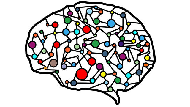
So far we have seen how basic calculations work in TensorFlow. The computational graph we have built actually resemble the biological neural network of human brain because of which it is commonly known as Artificial Neural Network or simply Neural Network.

The neurons in a neural network are organized across three types of layers:

1. Input Layer: This layer is used to feed the input data (features) into the network. There can be only one input layer in a network.
2. Output Layer: This layer holds the final output result after the computational graph is executed. The output can be a single value for regression problems or could be multiple values for classification problems. There can be only one output layer in a network.
3. Hidden Layers: This layer process the input from input layer and delivers the final result(s) to the output layer. This layer is where all the weights of the equation are derived. There can be multiple hidden layers in a network.

Neural Network

The two main problems with hidden layers is determining the total number of hidden layers and number of neurons in each layer. If we keep high number of neurons and layers then besides making the computation very expensive we will also start to see the problem of overfitting with respect to training data. On the other hand, if we don’t provide enough neurons then our model might not be effective enough to handle the complexity of the input data.

ACTIVATION FUNCTION

In the TensorFlow blog we have seen that the input parameters are multiplied by the weights and a bias is added to arrive at the final output. These kinds of linear equations are generally not adequate to resemble the complexities of real world data sets. The neural networks need to be able to compute any function that is why they are also known as Universal Function Approximators. The non-linearity to these equations is added by passing the output of the node through a function called Activation Function.

Additionally, the activation functions need to be also differentiable function which means there derivative exists for each point in its domain. Consequently, the graph of such a function is relatively smooth without any breaks, bends or cusps which makes it possible to move along the graph values for optimization during back propagation.

Some of the common activation functions are:

1. Sigmoid (Logistic): The output varies from 0 to 1. Main problem is with Vanishing Gradient Descent as the largest of values get condensed within a short range leading to no or negligible change in the gradient with iterations. Secondly it is not zero centered which doesn’t keep the gradient changes centered
2. TanH: The output varies from -1 to 1 so it is a zero centered function but it still suffers from Vanishing Gradient Descent problem
3. Rectified Linear Unit (ReLu): The output of this function varies from 0 to ∞. Since the values can vary till ∞ and not get constrained in small range it doesn’t have the Vanishing Gradient Descent issue.

For regression problems we get an output value but for classification problems we need to map the output against a set of possible classes. Following are some common functions used for them:

1. Softmax: It is used for classification problems as it distributes the probability values from 0 to 1 for all the possible outcomes such that the sum of all probability values is 1. Then using an argmax function we can find the class having maximum probability amongst the possible outcomes.
2. Sigmoid: It can be used for binary classification problems.

In next blog let’s look at the practical implementation of neural network using the Hello World data set of Deep Learning world called MNIST which is a handwritten digit recognition problem.